Pulling Hi-C data with mariner

Eric Davis

2024-04-08

mariner offers 2 functions for extracting/pulling interactions from .hic files - pullHicPixels() and pullHicMatrices(). In this article, you will learn how to extract Hi-C pixels or count matrices and access them from the resulting objects.

pullHicPixels() and pullHicMatrices() accept the same set of arguments, but return different outputs. Which function you choose depends on whether you want to extract a single value for each interaction or a matrix of values between a range of interactions.

When to use pullHicPixels()

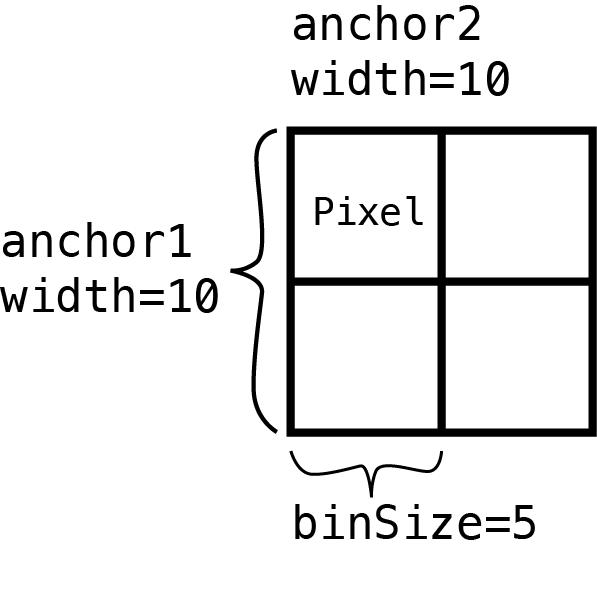
If you want a single value for each interaction and .hic file then you should use the pullHicPixels() function. We define a “pixel” as an interaction where both anchors are the same width. The binSize argument is used here to check that your desired pixel resolution matches your input interactions.

Note

You can check your .hic file to see which resolutions are available for the binSize argument with the strawr::readHicBpResolutions(). See the assignToBins() to set your interactions to an acceptable resolution.

The following example pulls 100-Kb pixels from two .hic files:

## Load mariner
library(mariner)

## Use example .hic files from ExperimentHub
hicFiles <- c(
    marinerData::LEUK_HEK_PJA27_inter_30.hic(),
    marinerData::LEUK_HEK_PJA30_inter_30.hic()
)
names(hicFiles) <- c("hic1", "hic2")

## Make some example interactions
gi <- read.table(
    text="
    1 51000000 51100000 1 51000000 51100000
    1 150000000 150100000 1 150000000 150100000
    2 51000000 51100000 2 51000000 51100000
    2 150000000 150100000 2 150000000 150100000
    "
)
gi <- as_ginteractions(gi)

## Pull Hi-C pixels
pixels <- pullHicPixels(x=gi, files=hicFiles, binSize=100e3)
pixels

## class: InteractionMatrix 
## dim: count matrix with 4 interactions and 2 file(s)
## metadata(3): binSize norm matrix
## assays(1): counts
## rownames: NULL
## rowData names(0):
## colnames(2): hic1 hic2
## colData names(2): files fileNames
## type: GInteractions
## regions: 4

This results in an InteractionMatrix object which contains the extracted Hi-C data, interactions, and metadata for the interactions and .hic files.

The extracted Hi-C data is stored as a count matrix where every row is an interaction (i.e pixel) and each column is a .hic file. Use the counts() function to access the count matrix from an InteractionMatrix object.

counts(pixels)

## <4 x 2> DelayedMatrix object of type "double":
##      hic1 hic2
## [1,]   53   49
## [2,]   63   56
## [3,]   36   16
## [4,]   43   24

This count matrix is stored on-disk (if onDisk=TRUE) as an HDF5-backed DelayedArray object. The data is stored in the provided file path to the h5File argument. If a file path isn’t provided, a temporary file is created in the current Rsession. To access or update the location of the HDF5 file after using the pullHicPixels() function, use the path() function.

path(pixels)

## [1] "/tmp/Rtmp5EwPyF/file1b52546e19d.h5"

Note

Using a DelayedArray instead of a normal R matrix has a number of benefits, especially for users working with limited computer memory. See the ?DelayedArray package documentation and vignettes for more information.

The count matrix can then be used for downstream analysis such as differential interaction analysis with DESeq2. To learn more about how to access components of InteractionMatrix objects, see the InteractionMatrix class section below.

When to use pullHicMatrices()

If you want a matrix of values for each interaction then you should use the pullHicMatrices() function. These matrices are made up of multiple “pixels”, defined by dividing the range of each interaction by the supplied binSize parameter.

Square matrices

For example, if you define 500x500 Kb interactions by setting the width of both anchors to be 500 Kb

## Create 500x500 Kb regions
regions <- assignToBins(x=gi, binSize=500e3, pos1="start", pos2="start")

Then set the binSize to 100 Kb

## Pull Hi-C matrices
matrices <- pullHicMatrices(x=regions, files=hicFiles, binSize=100e3)
matrices

## class: InteractionArray 
## dim: 4 interaction(s), 2 file(s), 5x5 count matrix(es)
## metadata(3): binSize norm matrix
## assays(3): counts rownames colnames
## rownames: NULL
## rowData names(0):
## colnames(2): hic1 hic2
## colData names(2): files fileNames
## type: GInteractions
## regions: 4

It produces count matrices each with 5 rows and 5 columns. These count matrices are stored in the InteractionArray class and are accessible with the counts() function.

counts(matrices)

## <5 x 5 x 4 x 2> DelayedArray object of type "double":
## ,,1,hic1
##      [,1] [,2] [,3] [,4] [,5]
## [1,]   53   15    5    1    4
## [2,]   15   68   19    8    5
## [3,]    5   19   69   12    2
## [4,]    1    8   12   48   13
## [5,]    4    5    2   13   48
## 
## ...
## 
## ,,4,hic2
##      [,1] [,2] [,3] [,4] [,5]
## [1,]   24   11    3    7    4
## [2,]   11   26    2    6    5
## [3,]    3    2   41   17    4
## [4,]    7    6   17   42   14
## [5,]    4    5    4   14   44

You can supply showDimnames=TRUE to display the start bin of each anchor.

counts(matrices, showDimnames=TRUE)

## <5 x 5 x 4 x 2> DelayedArray object of type "double":
## ,,1,hic1
##          51000000 51100000 51200000 51300000 51400000
## 51000000       53       15        5        1        4
## 51100000       15       68       19        8        5
## 51200000        5       19       69       12        2
## 51300000        1        8       12       48       13
## 51400000        4        5        2       13       48
## 
## ...
## 
## ,,4,hic2
##           150000000 150100000 150200000 150300000 150400000
## 150000000        24        11         3         7         4
## 150100000        11        26         2         6         5
## 150200000         3         2        41        17         4
## 150300000         7         6        17        42        14
## 150400000         4         5         4        14        44

These 4-dimensional arrays use the first and second dimensions as the rows and columns of the count matrices, the third dimension for each interaction, and the fourth dimension for each .hic file.

If you want to convert pixels to square Hi-C regions, you can use the pixelsToMatrices() function. The buffer argument describes how many pixels to expand the ranges on either side of the center pixel. For example, to expand 100x100 Kb pixels to regions that are 500x500 Kb, specify buffer=2 to add two additional 100 Kb pixels on both sides of the central 100 Kb pixels.

regions <- pixelsToMatrices(x=gi, buffer=2)
IRanges::width(regions)

## $first
## [1] 500001 500001 500001 500001
## 
## $second
## [1] 500001 500001 500001 500001

When pulled with pullHicMatrices() using binSize=100e3 odd, 5x5 matrices result.

pullHicMatrices(x=regions, files=hicFiles, binSize=100e3)

## class: InteractionArray 
## dim: 4 interaction(s), 2 file(s), 5x5 count matrix(es)
## metadata(3): binSize norm matrix
## assays(3): counts rownames colnames
## rownames: NULL
## rowData names(0):
## colnames(2): hic1 hic2
## colData names(2): files fileNames
## type: GInteractions
## regions: 4

Rectangular matrices

The previous example returns square count matrices where the width of both anchors are the same for each interaction. mariner also supports rectangular count matrices where the widths of the rows and columns are not equal.

For example, you can define 300x600 Kb interactions by setting the width of the first anchor to be 300 Kb and the second anchor to be 600 Kb.

## Create 300x600 Kb regions
regions <- assignToBins(
    x=gi,
    binSize=c(300e3, 600e3),
    pos1="start",
    pos2="start"
)

Then set the binSize to 100 Kb

## Pull Hi-C matrices
matrices <- pullHicMatrices(x=regions, files=hicFiles, binSize=100e3)
matrices

## class: InteractionArray 
## dim: 4 interaction(s), 2 file(s), 3x6 count matrix(es)
## metadata(3): binSize norm matrix
## assays(3): counts rownames colnames
## rownames: NULL
## rowData names(0):
## colnames(2): hic1 hic2
## colData names(2): files fileNames
## type: GInteractions
## regions: 8

Which produces an InteractionArray object with count matrices each with 3 rows and 6 columns.

counts(matrices, showDimnames=TRUE)

## <3 x 6 x 4 x 2> DelayedArray object of type "double":
## ,,1,hic1
##          51000000 51100000 51200000 51300000 51400000 51500000
## 51000000       53       15        5        1        4        1
## 51100000       15       68       19        8        5        5
## 51200000        5       19       69       12        2        2
## 
## ...
## 
## ,,4,hic2
##           150000000 150100000 150200000 150300000 150400000 150500000
## 150000000        24        11         3         7         4         1
## 150100000        11        26         2         6         5         0
## 150200000         3         2        41        17         4         9

Extracting square and rectangular matrices of data results in InteractionArray objects. See InteractionArray class to learn more about accessing data from these objects.

Variable matrices

mariner also supports extracting count matrices that are different dimensions for each interaction.

For example, these three interactions have dimensions of 1x3, 3x3, and 3x2 after pulling matrices with a binSize of 100e3:

## Interactions of different dimensions
regions <- read.table(
    text="
    1 51000000 51100000 1 51000000 51300000
    1 150000000 150300000 1 150000000 150300000
    2 51000000 51300000 2 51000000 51200000
    "
)
regions <- as_ginteractions(regions)

## Pull Hi-C matrices
matrices <- pullHicMatrices(x=regions, files=hicFiles, binSize=100e3)
matrices

## class: InteractionJaggedArray
## dim: 3 interaction(s), 2 file(s), variable count matrix(es)
## metadata(3): binSize, norm, matrix
## colData: hic1, hic2
## colData names(2): files, fileNames
## HDF5: /tmp/Rtmp5EwPyF/file1b525c4209bc.h5

The resulting object is of class InteractionJaggedArray. The class is different than the previous examples because the classes that InteractionArray inherits from are designed for regular, rectangular data types. A custom class called JaggedArray is used to hold irregular, or jagged, arrays of data.

The same counts() function returns these JaggedArray objects containing the Hi-C count data for each interaction and .hic file.

counts(matrices)

## <n x m x 3 x 2> JaggedArray:
## ,,1,1
## <1 x 3> matrix
##      [,1] [,2] [,3]
## [1,]   53   15    5
## 
## ...
## 
## ,,3,2
## <3 x 2> matrix
##      [,1] [,2]
## [1,]   16    6
## [2,]    6   17
## [3,]    3    7

See the InteractionJaggedArray class section to learn more about accessing and transforming data from InteractionJaggedArray and JaggedArray objects.

InteractionMatrix class

The InteractionMatrix class extends the InteractionSet and SummarizedExperiment classes. Therefore, it also inherits the accessors and methods of these objects. For example, you can access the original interactions, metadata about the experiment, row or column metadata, and subset or index slices of these objects. The following sections highlight some of the most useful accessors and methods for InteractionMatrix using this example object:

## Load mariner
library(mariner)

## Use example .hic files from ExperimentHub
hicFiles <- c(
    marinerData::LEUK_HEK_PJA27_inter_30.hic(),
    marinerData::LEUK_HEK_PJA30_inter_30.hic()
)
names(hicFiles) <- c("hic1", "hic2")

## Make some example interactions
gi <- read.table(
    text="
    1 51000000 51100000 1 51000000 51100000
    1 150000000 150100000 1 150000000 150100000
    2 51000000 51100000 2 51000000 51100000
    2 150000000 150100000 2 150000000 150100000
    "
)
gi <- as_ginteractions(gi)

## InteractionMatrix
imat <- pullHicPixels(x=gi, files=hicFiles, binSize=100e3)

Common accessors

## Show method
imat

## class: InteractionMatrix 
## dim: count matrix with 4 interactions and 2 file(s)
## metadata(3): binSize norm matrix
## assays(1): counts
## rownames: NULL
## rowData names(0):
## colnames(2): hic1 hic2
## colData names(2): files fileNames
## type: GInteractions
## regions: 4

## Dimensions
dim(imat)

## [1] 4 2

## Metadata about Hi-C extraction
metadata(imat)

## $binSize
## [1] 1e+05
## 
## $norm
## [1] "NONE"
## 
## $matrix
## [1] "observed"

## Metadata about interactions
SummarizedExperiment::rowData(imat)

## DataFrame with 4 rows and 0 columns

## Metadata about columns
SummarizedExperiment::colData(imat)

## DataFrame with 2 rows and 2 columns
##                       files         fileNames
##                 <character>       <character>
## hic1 /home/runner/.cache/.. 17dd605ffcd1_8147
## hic2 /home/runner/.cache/.. 17dd2067e2b6_8148

## Interactions
interactions(imat)

## GInteractions object with 4 interactions and 0 metadata columns:
##       seqnames1             ranges1     seqnames2             ranges2
##           <Rle>           <IRanges>         <Rle>           <IRanges>
##   [1]         1   51000000-51100000 ---         1   51000000-51100000
##   [2]         1 150000000-150100000 ---         1 150000000-150100000
##   [3]         2   51000000-51100000 ---         2   51000000-51100000
##   [4]         2 150000000-150100000 ---         2 150000000-150100000
##   -------
##   regions: 4 ranges and 0 metadata columns
##   seqinfo: 2 sequences from an unspecified genome; no seqlengths

## Count matrices
counts(imat)

## <4 x 2> DelayedMatrix object of type "double":
##      hic1 hic2
## [1,]   53   49
## [2,]   63   56
## [3,]   36   16
## [4,]   43   24

Indexing and subsetting

You can subset the interactions and files of the object directly where the first position subsets interactions and the second subsets files.

imat[1:3] |> counts()

## <3 x 2> DelayedMatrix object of type "double":
##      hic1 hic2
## [1,]   53   49
## [2,]   63   56
## [3,]   36   16

imat[3:1] |> counts()

## <3 x 2> DelayedMatrix object of type "double":
##      hic1 hic2
## [1,]   36   16
## [2,]   63   56
## [3,]   53   49

imat[,2] |> counts()

## <4 x 1> DelayedMatrix object of type "double":
##      hic2
## [1,]   49
## [2,]   56
## [3,]   16
## [4,]   24

imat[1,1] |> counts()

## <1 x 1> DelayedMatrix object of type "double":
##      hic1
## [1,]   53

Concatenating

Use the rbind() or cbind() functions to combine interactions row-wise or column-wise, respectively.

cbind(imat[,1], imat[,2])

## class: InteractionMatrix 
## dim: count matrix with 4 interactions and 2 file(s)
## metadata(3): binSize norm matrix
## assays(1): counts
## rownames: NULL
## rowData names(0):
## colnames(2): hic1 hic2
## colData names(2): files fileNames
## type: GInteractions
## regions: 4

rbind(imat[1:2,], imat[3:4,])

## class: InteractionMatrix 
## dim: count matrix with 4 interactions and 2 file(s)
## metadata(3): binSize norm matrix
## assays(1): counts
## rownames: NULL
## rowData names(0):
## colnames(2): hic1 hic2
## colData names(2): files fileNames
## type: GInteractions
## regions: 4

Note that the column metadata must be the same when using rbind and the row interactions must be the same when using cbind.

rbind(imat[1:2,1], imat[3:4,2])

## Error in `rbind()`:
## ! Can't rbind InteractionMatrix objects with different colData.

cbind(imat[1:2,1], imat[3:4,2])

## Error in `cbind()`:
## ! interactions must be identical in 'cbind'

Overlapping

Methods for subsetByOverlaps(), findOverlaps(), countOverlaps(), and overlapsAny() are inherited from the InteractionSet and IRanges packages. See the documentation and vignettes of these packages for usage and behavior of these functions.

InteractionArray class

The InteractionArray class extends the InteractionSet and SummarizedExperiment classes. Therefore, it also inherits the accessors and methods of these objects. For example, you can access the original interactions, metadata about the experiment, row or column metadata, and subset or index slices of these objects. Unlike the the InteractionMatrix class which returns an “interaction-by-Hi-C” matrix, the InteractionArray class returns count matrices for each interaction and .hic file. This results in a 4-dimensional array, where the first two dimensions are the rows and columns of the count matrices, the third dimension is the supplied interactions, and the fourth dimension is the supplied .hic files. This is stored as a DelayedArray which is accessible via the counts() accessor. The following sections highlight some of the most useful accessors and methods for InteractionMatrix using this example object:

## Load mariner
library(mariner)

## Use example .hic files from ExperimentHub
hicFiles <- c(
    marinerData::LEUK_HEK_PJA27_inter_30.hic(),
    marinerData::LEUK_HEK_PJA30_inter_30.hic()
)
names(hicFiles) <- c("hic1", "hic2")

## Create 500x500 Kb regions
regions <- read.table(
    text="
    1 51000000 51500000 1 51000000 51500000
    1 150000000 150500000 1 150000000 150500000
    2 51000000 51500000 2 51000000 51500000
    2 150000000 150500000 2 150000000 150500000
    "
)
regions <- as_ginteractions(regions)

## InteractionArray
ia <- pullHicMatrices(x=regions, files=hicFiles, binSize=100e3)

Common accessors

## Show method
ia

## class: InteractionArray 
## dim: 4 interaction(s), 2 file(s), 5x5 count matrix(es)
## metadata(3): binSize norm matrix
## assays(3): counts rownames colnames
## rownames: NULL
## rowData names(0):
## colnames(2): hic1 hic2
## colData names(2): files fileNames
## type: GInteractions
## regions: 4

## Dimensions
dim(ia)

## [1] 4 2

## Metadata about Hi-C extraction
metadata(ia)

## $binSize
## [1] 1e+05
## 
## $norm
## [1] "NONE"
## 
## $matrix
## [1] "observed"

## Metadata about interactions
SummarizedExperiment::rowData(ia)

## DataFrame with 4 rows and 0 columns

## Metadata about columns
SummarizedExperiment::colData(ia)

## DataFrame with 2 rows and 2 columns
##                       files         fileNames
##                 <character>       <character>
## hic1 /home/runner/.cache/.. 17dd605ffcd1_8147
## hic2 /home/runner/.cache/.. 17dd2067e2b6_8148

## Interactions
interactions(ia)

## GInteractions object with 4 interactions and 0 metadata columns:
##       seqnames1             ranges1     seqnames2             ranges2
##           <Rle>           <IRanges>         <Rle>           <IRanges>
##   [1]         1   51000000-51500000 ---         1   51000000-51500000
##   [2]         1 150000000-150500000 ---         1 150000000-150500000
##   [3]         2   51000000-51500000 ---         2   51000000-51500000
##   [4]         2 150000000-150500000 ---         2 150000000-150500000
##   -------
##   regions: 4 ranges and 0 metadata columns
##   seqinfo: 2 sequences from an unspecified genome; no seqlengths

## Count matrices
counts(ia)

## <5 x 5 x 4 x 2> DelayedArray object of type "double":
## ,,1,hic1
##      [,1] [,2] [,3] [,4] [,5]
## [1,]   53   15    5    1    4
## [2,]   15   68   19    8    5
## [3,]    5   19   69   12    2
## [4,]    1    8   12   48   13
## [5,]    4    5    2   13   48
## 
## ...
## 
## ,,4,hic2
##      [,1] [,2] [,3] [,4] [,5]
## [1,]   24   11    3    7    4
## [2,]   11   26    2    6    5
## [3,]    3    2   41   17    4
## [4,]    7    6   17   42   14
## [5,]    4    5    4   14   44

## Counts with start bins for anchor1 and 2
counts(ia, showDimnames=TRUE)

## <5 x 5 x 4 x 2> DelayedArray object of type "double":
## ,,1,hic1
##          51000000 51100000 51200000 51300000 51400000
## 51000000       53       15        5        1        4
## 51100000       15       68       19        8        5
## 51200000        5       19       69       12        2
## 51300000        1        8       12       48       13
## 51400000        4        5        2       13       48
## 
## ...
## 
## ,,4,hic2
##           150000000 150100000 150200000 150300000 150400000
## 150000000        24        11         3         7         4
## 150100000        11        26         2         6         5
## 150200000         3         2        41        17         4
## 150300000         7         6        17        42        14
## 150400000         4         5         4        14        44

Indexing and subsetting

You can subset the interactions and files of the object directly where the first position subsets interactions and the second subsets files.

ia[1:3] |> counts()

## <5 x 5 x 3 x 2> DelayedArray object of type "double":
## ,,1,hic1
##      [,1] [,2] [,3] [,4] [,5]
## [1,]   53   15    5    1    4
## [2,]   15   68   19    8    5
## [3,]    5   19   69   12    2
## [4,]    1    8   12   48   13
## [5,]    4    5    2   13   48
## 
## ...
## 
## ,,3,hic2
##      [,1] [,2] [,3] [,4] [,5]
## [1,]   16    6    3    2    4
## [2,]    6   17    7    2    0
## [3,]    3    7   23    6    0
## [4,]    2    2    6   23    2
## [5,]    4    0    0    2   24

ia[3:1] |> counts()

## <5 x 5 x 3 x 2> DelayedArray object of type "double":
## ,,1,hic1
##      [,1] [,2] [,3] [,4] [,5]
## [1,]   36    5    5    2    4
## [2,]    5   30   13    4    1
## [3,]    5   13   22    6    6
## [4,]    2    4    6   30    4
## [5,]    4    1    6    4   21
## 
## ...
## 
## ,,3,hic2
##      [,1] [,2] [,3] [,4] [,5]
## [1,]   49   27    4    5    3
## [2,]   27   49   13    2    6
## [3,]    4   13   56    7    8
## [4,]    5    2    7   48   10
## [5,]    3    6    8   10   47

ia[,2] |> counts()

## <5 x 5 x 4 x 1> DelayedArray object of type "double":
## ,,1,hic2
##      [,1] [,2] [,3] [,4] [,5]
## [1,]   49   27    4    5    3
## [2,]   27   49   13    2    6
## [3,]    4   13   56    7    8
## [4,]    5    2    7   48   10
## [5,]    3    6    8   10   47
## 
## ...
## 
## ,,4,hic2
##      [,1] [,2] [,3] [,4] [,5]
## [1,]   24   11    3    7    4
## [2,]   11   26    2    6    5
## [3,]    3    2   41   17    4
## [4,]    7    6   17   42   14
## [5,]    4    5    4   14   44

ia[1,1] |> counts()

## <5 x 5 x 1 x 1> DelayedArray object of type "double":
## ,,1,hic1
##      [,1] [,2] [,3] [,4] [,5]
## [1,]   53   15    5    1    4
## [2,]   15   68   19    8    5
## [3,]    5   19   69   12    2
## [4,]    1    8   12   48   13
## [5,]    4    5    2   13   48

Subsetting and indexing can also be done on the DelayedArray object accessed with counts(). For example, the following code shows how you could access the top left corner of the count matrix of the first interaction and .hic file.

counts(ia)[1:3, 1:3, 1, 1]

## <3 x 3> DelayedMatrix object of type "double":
##      [,1] [,2] [,3]
## [1,]   53   15    5
## [2,]   15   68   19
## [3,]    5   19   69

Concatenating

Use the rbind() or cbind() functions to combine interactions row-wise or column-wise, respectively.

cbind(ia[,1], ia[,2])

## class: InteractionArray 
## dim: 4 interaction(s), 2 file(s), 5x5 count matrix(es)
## metadata(3): binSize norm matrix
## assays(3): counts rownames colnames
## rownames: NULL
## rowData names(0):
## colnames(2): hic1 hic2
## colData names(2): files fileNames
## type: GInteractions
## regions: 4

rbind(ia[1:2,], ia[3:4,])

## class: InteractionArray 
## dim: 4 interaction(s), 2 file(s), 5x5 count matrix(es)
## metadata(3): binSize norm matrix
## assays(3): counts rownames colnames
## rownames: NULL
## rowData names(0):
## colnames(2): hic1 hic2
## colData names(2): files fileNames
## type: GInteractions
## regions: 4

Note that the column metadata must be the same when using rbind and the row interactions must be the same when using cbind.

rbind(ia[1:2,1], ia[3:4,2])

## Error in `rbind()`:
## ! Can't rbind InteractionArray objects with different colData.

cbind(ia[1:2,1], ia[3:4,2])

## Error in `cbind()`:
## ! interactions must be identical in 'cbind'

Overlapping

Methods for subsetByOverlaps(), findOverlaps(), countOverlaps(), and overlapsAny() are inherited from the InteractionSet and IRanges packages. See the documentation and vignettes of these packages for usage and behavior of these functions.

InteractionJaggedArray class

The InteractionJaggedArray class is a new class designed for holding irregularly sized count matrices, also known as “ragged” or “jagged” arrays along with other important information about the extracted Hi-C data. The count matrices are managed by the JaggedArray class which is analogous to the DelayedArray class. JaggedArray data is stored on-disk in an HDF5 file, and subsetting/indexing operations are delayed similarly to DelayedArray. Continue reading to learn about how to use InteractionJaggedArray and JaggedArray objects, and how to convert them to InteractionArray or DelayedArray objects with the regularize() function for downstream analysis.

## Load mariner
library(mariner)

## Use example .hic files from ExperimentHub
hicFiles <- c(
    marinerData::LEUK_HEK_PJA27_inter_30.hic(),
    marinerData::LEUK_HEK_PJA30_inter_30.hic()
)
names(hicFiles) <- c("hic1", "hic2")

## Create regions of different dimensions
regions <- read.table(
    text="
    1 51000000 51100000 1 51000000 51300000
    1 150000000 150300000 1 150000000 150300000
    2 51000000 51300000 2 51000000 51200000
    "
)
regions <- as_ginteractions(regions)

## InteractionJaggedArray
ija <- pullHicMatrices(x=regions, files=hicFiles, binSize=100e3)

Common accessors

## Show method
ija

## class: InteractionJaggedArray
## dim: 3 interaction(s), 2 file(s), variable count matrix(es)
## metadata(3): binSize, norm, matrix
## colData: hic1, hic2
## colData names(2): files, fileNames
## HDF5: /tmp/Rtmp5EwPyF/file1b526bd226a3.h5

The variable dimensions of the jagged arrays can be accessed with the dim() function:

## Dimensions
dim(ija)

## $interactions
## [1] 3
## 
## $files
## [1] 2
## 
## $rows
## [1] 1 3 3
## 
## $cols
## [1] 3 3 2

## Metadata about Hi-C extraction
metadata(ija)

## $binSize
## [1] 1e+05
## 
## $norm
## [1] "NONE"
## 
## $matrix
## [1] "observed"

## Metadata about columns
SummarizedExperiment::colData(ija)

## DataFrame with 2 rows and 2 columns
##                       files         fileNames
##                 <character>       <character>
## hic1 /home/runner/.cache/.. 17dd605ffcd1_8147
## hic2 /home/runner/.cache/.. 17dd2067e2b6_8148

## Access HDF5 filepath
path(ija)

## [1] "/tmp/Rtmp5EwPyF/file1b526bd226a3.h5"

## Interactions
interactions(ija)

## GInteractions object with 3 interactions and 0 metadata columns:
##       seqnames1             ranges1     seqnames2             ranges2
##           <Rle>           <IRanges>         <Rle>           <IRanges>
##   [1]         1   51000000-51100000 ---         1   51000000-51300000
##   [2]         1 150000000-150300000 ---         1 150000000-150300000
##   [3]         2   51000000-51300000 ---         2   51000000-51200000
##   -------
##   regions: 5 ranges and 0 metadata columns
##   seqinfo: 2 sequences from an unspecified genome; no seqlengths

The counts() function returns a JaggedArray

## Count matrices as JaggedArray
ja <- counts(ija)
ja

## <n x m x 3 x 2> JaggedArray:
## ,,1,1
## <1 x 3> matrix
##      [,1] [,2] [,3]
## [1,]   53   15    5
## 
## ...
## 
## ,,3,2
## <3 x 2> matrix
##      [,1] [,2]
## [1,]   16    6
## [2,]    6   17
## [3,]    3    7

This can be converted to a nested R list with the as.list() function, where the outer level refers to the .hic file and the inner level contains a matrix for each interaction.

as.list(ja)

## [[1]]
## [[1]][[1]]
##      [,1] [,2] [,3]
## [1,]   53   15    5
## 
## [[1]][[2]]
##      [,1] [,2] [,3]
## [1,]   63   25   15
## [2,]   25   68   28
## [3,]   15   28   87
## 
## [[1]][[3]]
##      [,1] [,2]
## [1,]   36    5
## [2,]    5   30
## [3,]    5   13
## 
## 
## [[2]]
## [[2]][[1]]
##      [,1] [,2] [,3]
## [1,]   49   27    4
## 
## [[2]][[2]]
##      [,1] [,2] [,3]
## [1,]   56   26    8
## [2,]   26   60   14
## [3,]    8   14   89
## 
## [[2]][[3]]
##      [,1] [,2]
## [1,]   16    6
## [2,]    6   17
## [3,]    3    7

Indexing and subsetting

You can subset the interactions and files of the object directly where the first position subsets interactions and the second subsets files.

ija[1:2] |> counts()

## <n x m x 2 x 2> JaggedArray:
## ,,1,1
## <1 x 3> matrix
##      [,1] [,2] [,3]
## [1,]   53   15    5
## 
## ...
## 
## ,,2,2
## <3 x 3> matrix
##      [,1] [,2] [,3]
## [1,]   56   26    8
## [2,]   26   60   14
## [3,]    8   14   89

ija[2:1] |> counts()

## <n x m x 2 x 2> JaggedArray:
## ,,1,1
## <3 x 3> matrix
##      [,1] [,2] [,3]
## [1,]   63   25   15
## [2,]   25   68   28
## [3,]   15   28   87
## 
## ...
## 
## ,,2,2
## <1 x 3> matrix
##      [,1] [,2] [,3]
## [1,]   49   27    4

ija[,2] |> counts()

## <n x m x 3 x 1> JaggedArray:
## ,,1,1
## <1 x 3> matrix
##      [,1] [,2] [,3]
## [1,]   49   27    4
## 
## ...
## 
## ,,3,1
## <3 x 2> matrix
##      [,1] [,2]
## [1,]   16    6
## [2,]    6   17
## [3,]    3    7

ija[1,1] |> counts()

## <1 x 3 x 1 x 1> DelayedArray object of type "double":
## ,,1,hic1
##      [,1] [,2] [,3]
## [1,]   53   15    5

Notice that when indexing results in subset of data with the same dimensions it is automatically coerced to an InteractionArray or DelayedArray.

ija[3,1] |> class()

## [1] "InteractionArray"
## attr(,"package")
## [1] "mariner"

ija[3,1] |> counts() |> class()

## [1] "DelayedArray"
## attr(,"package")
## [1] "DelayedArray"

You can also subset and index on the JaggedArray object by selecting the desired interactions(s) in the third dimension and .hic file(s) in the fourth dimension. Since the first two dimensions are variable, subsetting/indexing these is not supported.

ja[,,3,2]

## <3 x 2 x 1 x 1> DelayedArray object of type "double":
## ,,1,1
##      [,1] [,2]
## [1,]   16    6
## [2,]    6   17
## [3,]    3    7

If the selection results in a DelayedArray then normal indexing rules apply:

ja[,,3,2][1:2,1,1,1]

## [1] 16  6

Concatenating

Concatenating InteractionJaggedArray and JaggedArray objects is not currently supported. If you need this functionality please post an issue to the mariner repository or (even better) submit a pull request with an implementation.

Overlapping

Methods for subsetByOverlaps(), findOverlaps(), countOverlaps(), and overlapsAny() are inherited from the InteractionSet and IRanges packages. See the documentation and vignettes of these packages for usage and behavior of these functions.

Converting to regular arrays

For downstream aggregation and visualization, it is helpful to convert irregular/jagged arrays to regular arrays. The regularize() function stretches and (optionally) scales the count matrices into the desired rectangular (or square) matrices with dimensions supplied to ndim. The function works on both InteractionJaggedArray and JaggedArray objects.

regularize(x=ija, ndim=c(3,3)) |> counts()

## / Reading and realizing block 1/3 of file 1/2 ... OK
## \ Processing it ... Loading required namespace: fields
## OK
## / Reading and realizing block 2/3 of file 1/2 ... OK
## \ Processing it ... OK
## / Reading and realizing block 3/3 of file 1/2 ... OK
## \ Processing it ... OK
## / Reading and realizing block 1/3 of file 2/2 ... OK
## \ Processing it ... OK
## / Reading and realizing block 2/3 of file 2/2 ... OK
## \ Processing it ... OK
## / Reading and realizing block 3/3 of file 2/2 ... OK
## \ Processing it ... OK

## <3 x 3 x 3 x 2> DelayedArray object of type "double":
## ,,1,hic1
##            [,1]       [,2]       [,3]
## [1,] 0.24200913 0.06849315 0.02283105
## [2,] 0.24200913 0.06849315 0.02283105
## [3,] 0.24200913 0.06849315 0.02283105
## 
## ,,2,hic1
##            [,1]       [,2]       [,3]
## [1,] 0.17796610 0.07062147 0.04237288
## [2,] 0.07062147 0.19209040 0.07909605
## [3,] 0.04237288 0.07909605 0.24576271
## 
## ,,3,hic1
##            [,1]       [,2]       [,3]
## [1,] 0.25531915 0.14539007 0.03546099
## [2,] 0.03546099 0.12411348 0.21276596
## [3,] 0.03546099 0.06382979 0.09219858
## 
## ,,1,hic2
##            [,1]       [,2]       [,3]
## [1,] 0.20416667 0.11250000 0.01666667
## [2,] 0.20416667 0.11250000 0.01666667
## [3,] 0.20416667 0.11250000 0.01666667
## 
## ,,2,hic2
##            [,1]       [,2]       [,3]
## [1,] 0.18604651 0.08637874 0.02657807
## [2,] 0.08637874 0.19933555 0.04651163
## [3,] 0.02657807 0.04651163 0.29568106
## 
## ,,3,hic2
##            [,1]       [,2]       [,3]
## [1,] 0.19393939 0.13333333 0.07272727
## [2,] 0.07272727 0.13939394 0.20606061
## [3,] 0.03636364 0.06060606 0.08484848

regularize(x=ja, ndim=c(3,3))

## / Reading and realizing block 1/3 of file 1/2 ... OK
## \ Processing it ... OK
## / Reading and realizing block 2/3 of file 1/2 ... OK
## \ Processing it ... OK
## / Reading and realizing block 3/3 of file 1/2 ... OK
## \ Processing it ... OK
## / Reading and realizing block 1/3 of file 2/2 ... OK
## \ Processing it ... OK
## / Reading and realizing block 2/3 of file 2/2 ... OK
## \ Processing it ... OK
## / Reading and realizing block 3/3 of file 2/2 ... OK
## \ Processing it ... OK

## <3 x 3 x 3 x 2> HDF5Array object of type "double":
## ,,1,1
##            [,1]       [,2]       [,3]
## [1,] 0.24200913 0.06849315 0.02283105
## [2,] 0.24200913 0.06849315 0.02283105
## [3,] 0.24200913 0.06849315 0.02283105
## 
## ,,2,1
##            [,1]       [,2]       [,3]
## [1,] 0.17796610 0.07062147 0.04237288
## [2,] 0.07062147 0.19209040 0.07909605
## [3,] 0.04237288 0.07909605 0.24576271
## 
## ,,3,1
##            [,1]       [,2]       [,3]
## [1,] 0.25531915 0.14539007 0.03546099
## [2,] 0.03546099 0.12411348 0.21276596
## [3,] 0.03546099 0.06382979 0.09219858
## 
## ,,1,2
##            [,1]       [,2]       [,3]
## [1,] 0.20416667 0.11250000 0.01666667
## [2,] 0.20416667 0.11250000 0.01666667
## [3,] 0.20416667 0.11250000 0.01666667
## 
## ,,2,2
##            [,1]       [,2]       [,3]
## [1,] 0.18604651 0.08637874 0.02657807
## [2,] 0.08637874 0.19933555 0.04651163
## [3,] 0.02657807 0.04651163 0.29568106
## 
## ,,3,2
##            [,1]       [,2]       [,3]
## [1,] 0.19393939 0.13333333 0.07272727
## [2,] 0.07272727 0.13939394 0.20606061
## [3,] 0.03636364 0.06060606 0.08484848

By using regularize() before extracting counts, you can take advantage of the block and parallel processing functionality from aggregating with aggHicMatrices():

regularize(x=ija, ndim=c(3,3), nBlocks=1) |>
    aggHicMatrices(nBlocks=1)

## / Reading and realizing block 1/1 of file 1/2 ... OK
## \ Processing it ... OK
## / Reading and realizing block 1/1 of file 2/2 ... OK
## \ Processing it ... OK
## / reading and realizing block 1/1 ... ok
## \ processing it ... ok

## <3 x 3> DelayedMatrix object of type "double":
##           [,1]      [,2]      [,3]
## [1,] 1.2594470 0.6167168 0.2166369
## [2,] 0.7113643 0.8359265 0.5839320
## [3,] 0.5869514 0.4310367 0.7579886

Other pullHic* arguments

The previous sections provided examples of using pullHicPixels() and pullHicMatrices(), for extracting Hi-C pixels and count matrices, respectively. These functions require three mandatory arguments: x for interactions, files for .hic file paths, and binSize for the Hi-C resolution.

Additionally, the remaining arguments allow for greater control over the Hi-C data extraction process. These arguments control the type of Hi-C data to be extracted, the efficiency of extraction, and specify the storage location for the extracted data.

In this section we delve deeper into the utilization of these arguments to effectively extract Hi-C data.

Normalization and matrix type

The norm and matrix arguments are passed to strawr during the extraction step.

norm refers to the Hi-C normalization and is limited to pre-computed normalizations in the .hic file. Use the readHicNormTypes() function from the strawr package to see available normalizations.

pullHicPixels(x=gi, files=hicFiles, binSize=100e3, norm="none")

## Error in `.checkStrawArgs()`:
## ! `norm` must be one of "NONE", "KR", "VC_SQRT", or "VC", not "none".
## ℹ Did you mean "NONE"?

The matrix argument specifies the type of values to extract. The default is the “observed” contact frequency values. Other options include “expected” contact frequency and the “oe” or observed/expected values. For an in-depth description of these matrix types see Durand et al. 2016

pullHicPixels(x=gi, files=hicFiles, binSize=100e3, matrix="oe") |>
    counts()

## <4 x 2> DelayedMatrix object of type "double":
##           hic1      hic2
## [1,] 1.0564467 1.1543123
## [2,] 1.2557763 1.3192140
## [3,] 0.9188343 0.5032488
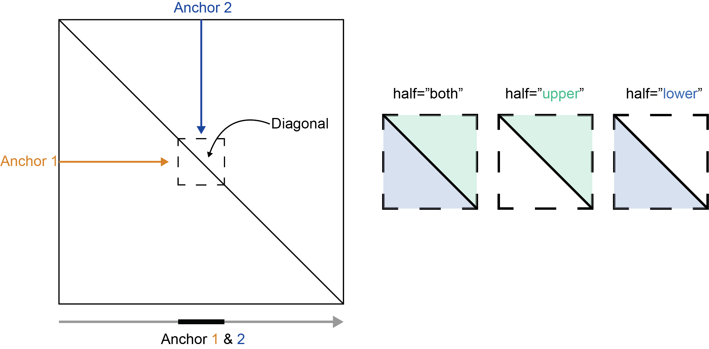
## [4,] 1.0974965 0.7548732

The half parameter

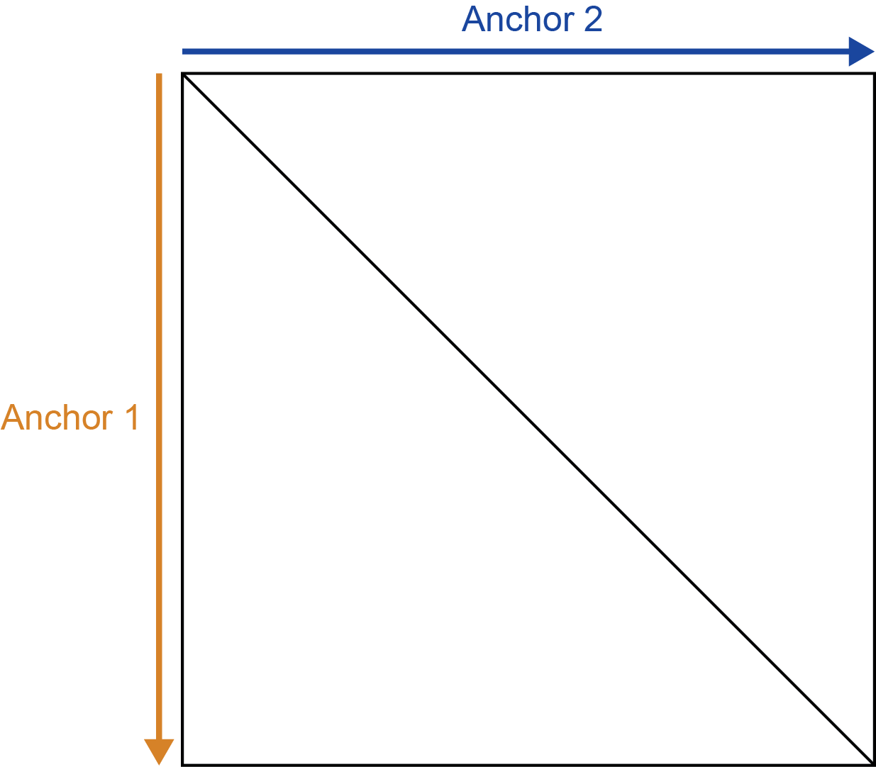
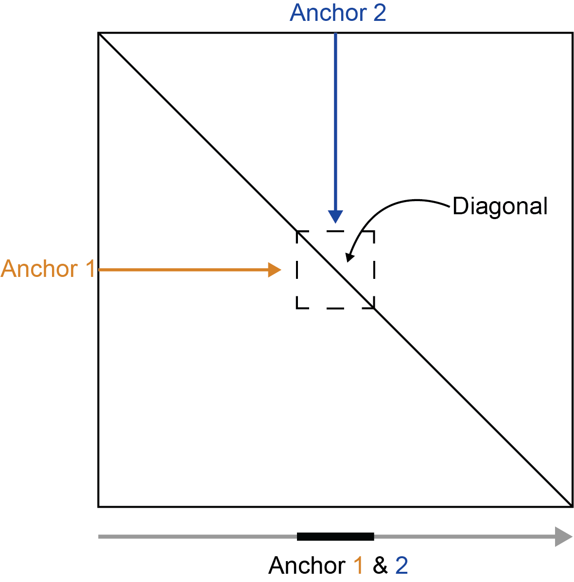
The Hi-C matrix is a square, symmetric matrix that captures the frequency of all pair-wise interactions between genomic loci. In other words, each point in a Hi-C matrix represents the interaction frequency between a two pairs, or anchors, of genomic regions.

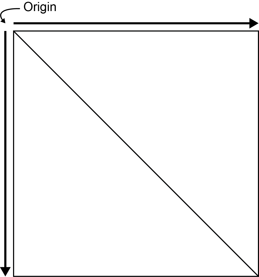
In mariner, the Hi-C matrix is oriented with the origin (lowest genomic coordinates) in the upper left corner with linear genomic position increasing down and to the right.

The first anchor, or genomic locus, corresponds on the vertical axis (rows of matrix) while the second anchor corresponds to the horizontal axis (columns of the matrix). Together, these anchors specify a two-dimensional region on the Hi-C matrix.

The relative positions of these anchors determines from which “half” of the matrix data is extracted. When the genomic position of the first anchor is less than the second anchor the region resides in the upper trianglar.

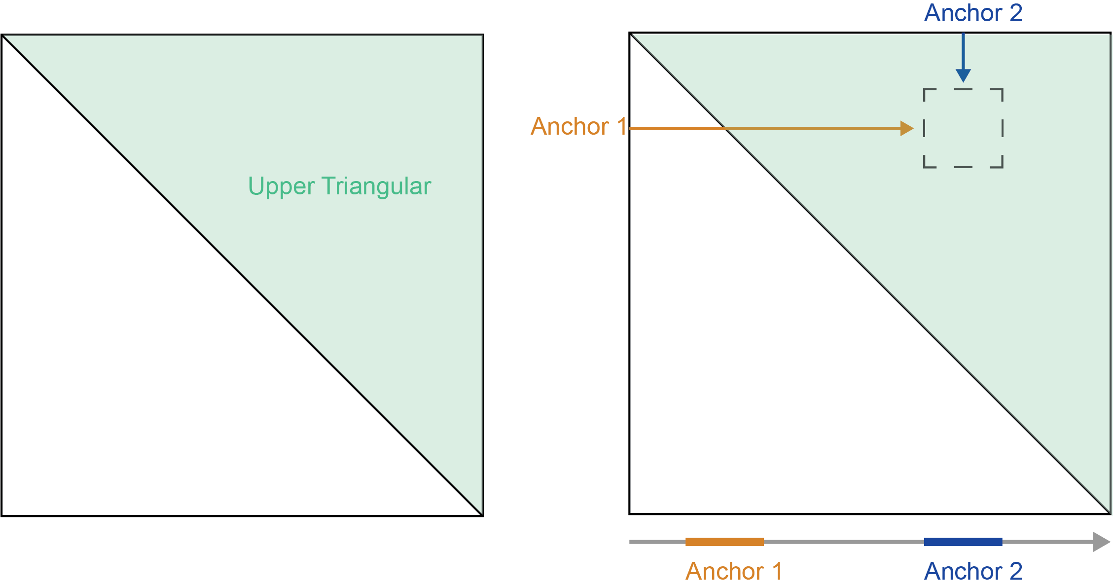
When the genomic position of the first anchor is greater than the second anchor the region resides in the lower triangular.

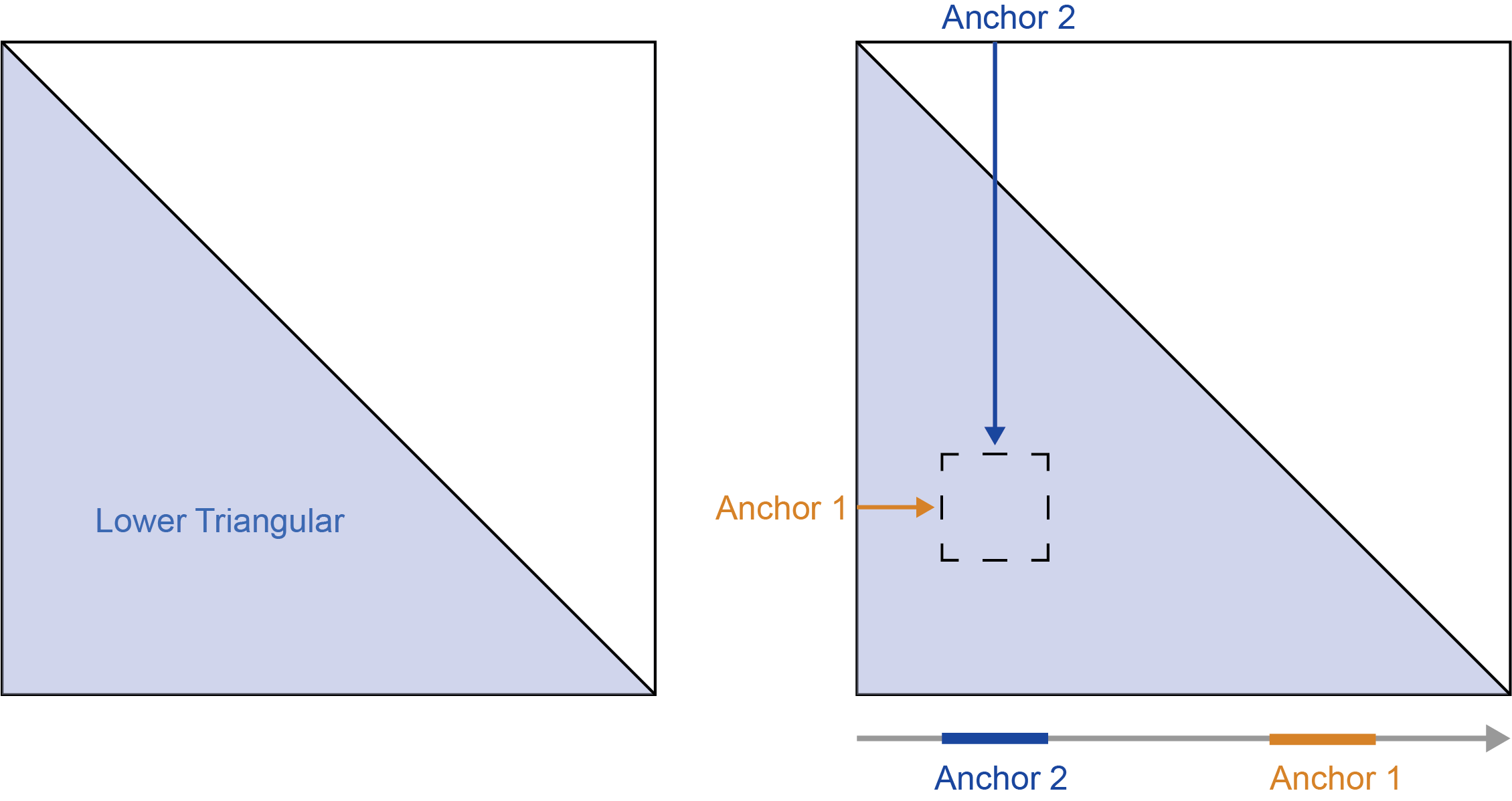
If the first and second anchors are equal then the region is on the diagonal and the values will be mirrored across the diagonal.

To summarize:

• first < second - upper triangular
• first > second - lower triangular
• first == second - mirrored diagonal

The half parameter controls which portion of the Hi-C matrix is returned, regardless of anchor position. When half="upper" only upper-triangular data is returned. When half="lower" only lower-triangular data is returned. half="both" returns upper and lower triangular data. NA values are returned for portions of the matrix that do not match the region of the matrix specified with half. The figure and code below show how data are returned for a region that resides on the diagonal, crossing into both the upper and lower triangular of the Hi-C matrix.

## Hic file
hic <- marinerData::LEUK_HEK_PJA27_inter_30.hic()

## On-diagonal interaction
diagonal <- as_ginteractions(read.table(text="
    1 51000000 51300000 1 51000000 51300000
"))

## half="upper"
pullHicMatrices(x=diagonal, files=hic, binSize=100e3, half="upper") |>
    counts()

## <3 x 3 x 1 x 1> DelayedArray object of type "double":
## ,,1,EH8088
##      [,1] [,2] [,3]
## [1,]   53   15    5
## [2,]   NA   68   19
## [3,]   NA   NA   69

## half="lower"
pullHicMatrices(x=diagonal, files=hic, binSize=100e3, half="lower") |>
    counts()

## <3 x 3 x 1 x 1> DelayedArray object of type "double":
## ,,1,EH8088
##      [,1] [,2] [,3]
## [1,]   53   NA   NA
## [2,]   15   68   NA
## [3,]    5   19   69

## half="both"
pullHicMatrices(x=diagonal, files=hic, binSize=100e3, half="both") |>
    counts()

## <3 x 3 x 1 x 1> DelayedArray object of type "double":
## ,,1,EH8088
##      [,1] [,2] [,3]
## [1,]   53   15    5
## [2,]   15   68   19
## [3,]    5   19   69

Since chromosomes have no inherent order in linear genomic space, the half parameter is ignored for interchromosomal interactions. pullHicPixels() behaves the same way with the half parameter.

Changing blockSize for large data

pullHicPixels() and pullHicMatrices() allow you to tune the efficiency and memory-usage of Hi-C data extraction by grouping nearby interactions into blocks. The block data is then loaded into memory, assigned to interactions, and then written to back to disk as an HDF5 file. You can modify the blockSize (in base-pairs) to control the size and number of blocks that are extracted. Pulling larger blocks decreases run-time, but requires more RAM to store these data while smaller blocks increase run-time, but allows you to extract counts from large Hi-C files that may not otherwise fit into memory.

Adjustments to blockSize can optimize the efficiency of extraction. There is a trade-off between the size of the block and the number of iterations required to extract all interactions. The size and placement of interactions on the genome also affects the blockSize. For example, a worst-case performance scenario would be extracting each interaction individually (setting blockSize to the width of the interaction). Generally, it is most efficient to extract the largest blocks possible. When your data is small enough, pulling whole chromosomes is usually most efficient. However, the optimal blockSize is highly dependent on both the interactions and .hic files, so you may want to experiment with this parameter to find the best trade-off for your data.

The compressionLevel and chunkSize parameters control the way extracted data is written back to the HDF5-file. See ?pullHicMatrices or ?pullHicPixels for a more in-depth description of these parameters.